Why Data Processing is instrumental in MMM projects, By MASS Analytics’ Dr. Ramla Jarrar

In the previous article, we covered Data Exploration which paved our way to the fifth article in our series. Now that the analyst is familiar with their charted data, in-depth work should be conducted to successfully transform the variables and test various hypotheses to get a better idea about the reality behind the model inputs.

This article explores a set of transformations that could be applied during the Data Processing phase.

The rationale behind Data Processing:

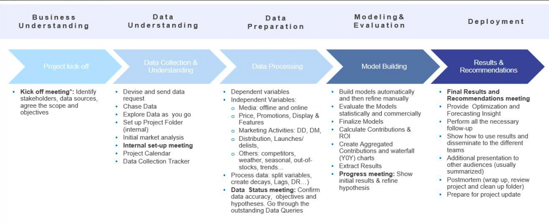
Data processing involves transforming raw data into useful formats that can be analyzed effectively. This phase comes third in the marketing mix modeling workflow:

The idea behind data processing is to create additional variables (they stem from Data Exploration). Those variables are then tested through the modeling stage, to either confirm or refute the hypothesis that had been established.

What types of variables could be created in Data Processing?

The new variables that the analyst could create at this stage are divided into two main groups:

Calendar variables: They are created from scratch. They are not based on raw variables that exist in the project. For example, dummies, or trends.
Processed variables: They are transformations applied to raw variables. For example, if decay is applied to a TV GRP, that results in a processed variable
Diminishing returns, lags, seasonality, adding up variables, and splitting variables are also examples of processed variables that we will explore in this article.

Let’s start Calendar variables:

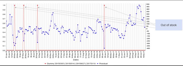
Dummy variables: They are generally created to model events, whether they are known or unknown. Analysts should be very careful when using dummy variables. The exaggerated and non explained used of dummy variables may result in an overfitted model.

Example: An out of stock, which happens 3 times a year, is a situation where 3 dummies could be added to the model to represent this event.

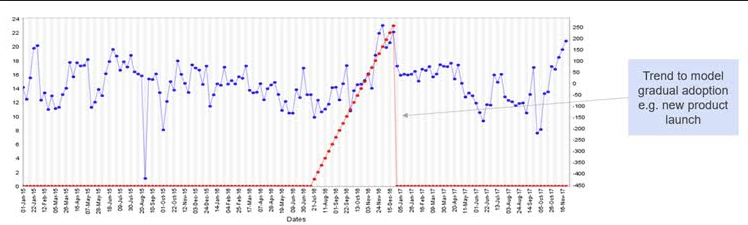
Trends and Part Trends: They are created to model the gradual increase, or decrease, in the modeled KPI. The delisting of a product is a case in point, and so is the launch of a new product, as illustrated in figure 3.
In the retail sector, it could be modeling the opening or the closure of a store.

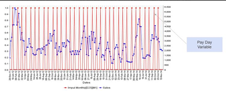
Periodic: This is generally used to model a frequent event, for example: Payday (figure 4). People get paid around the 25th of the month; so, an increase in consumption is expected.  In this case, the analyst could create a variable that takes the value “1” on the week where the 25th of every month falls. This could be done using the Periodic transformation.

Another example is seasonality during a specific month of the year such as June. Here, a periodic seasonality in June could be created. And if the data modeled is over the course of three years, we will end up with three sequences of those using the periodic transformation.

Processed variables:

Processed variables are created either out of the raw variables that are already collected as part of the kickoff meeting and the data request, or out of the Calendar Variables. What is advisable before creating any processed variables, is to graph the raw variable against the dependent variable. Based on the comparison, the analyst should choose the transformations that would be adapted to the raw variable. This leads them to creating the shape that they are aiming to model at a later stage. These transformations include:

Decay is one of the most popular transformations in Marketing Mix Modeling. It is commonly called Adstock. The theory behind it is as simple as saying that there is a prolonged (or carry-over) effect of the advertising activity. So, when the business advertises at a time “t”, that activity will not have an impact on consumption only at time “t”. It will also carry over to the following weeks. Mathematically, it is perceived as a stock of advertising that is influenced by two factors:

1: How much activity, or how much advertising, the consumer is exposed to in that particular week.

2: A carryover effect that is coming from the stock of advertising from previous weeks.

Decay will determine how much memory the consumer takes with them week after week.

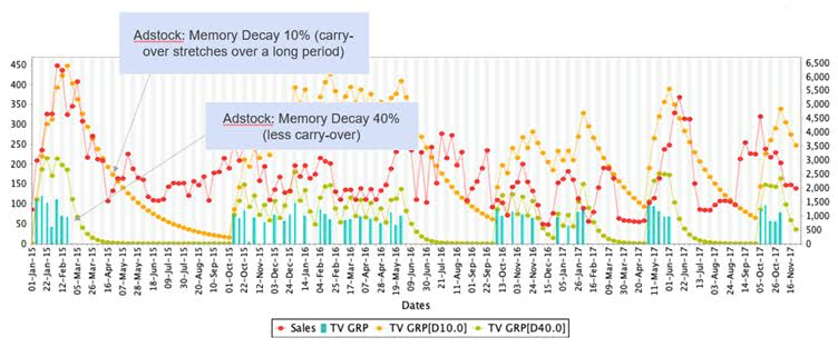
The following is an illustration of the Ad Stock concept:

The dependent variable is graphed in red
The raw TV GRP is graphed in blue.

Two types of Adstock were created here:

In the first one, which is yellow, we are assuming a memory decay of 10%. Here, the carryover stretches over a long period because the consumer only forgets 10% of the message they have been exposed to.

That means 90% of the message is taken over week on week.

In the second transformation, which is the 40%, the stock of advertising that is taken over week on week is less than in the first case of 10%.

It is noticeable that the green line falls probably two or three weeks following the end the TV activity.

The idea behind Adstock is to create different variations of Decay. Then when the analyst moves to the modeling stage, they choose the best variable that best matches the variations seen in sales.

How do we determine where to stop the Decay?

Another variation of the decay function is to specify a Cutoff point. It means that the user decides to stop the tail starting from a certain point. So, all what they need to do is to enter the cutoff point, and the software they use should be able to automatically creates 2 variables:

One before the cutoff point to measure the short-term effect
Another after the cutoff point to measure medium/long term effect

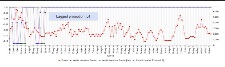
Lag: It is generally applied to shift a variable to model its delayed effect. A good example of this is promotions (see figure 5): what one would expect is that when promotions are on, sales would be increasing as a result. However, depending on the strength of the promotion, that could easily result in a drop in sales in subsequent weeks. Let’s take the case of “buy one get one free”, what generally tends to happen is that customers will stock the products they buy in times of promotion. Consequently, they won’t do their shopping as usual in the subsequent weeks. 

What the analyst needs to do here is create a lag of the promotion variable. While the raw variable of promotion will be used to model the immediate effect of promotions, the lagged version will be used to model the brought forward sales, as well as a potential decrease in the sales line.

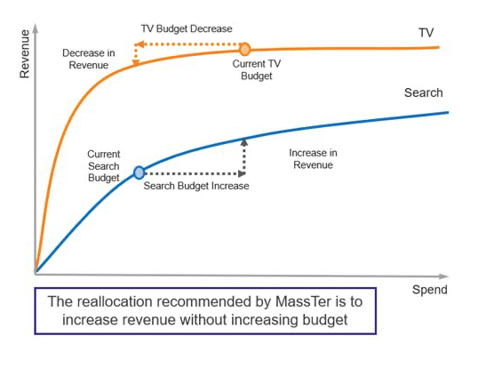
Diminishing Returns: It is one of the most important transformations in the context of Marketing Mix Modeling. If the purpose is to create an optimization as part of the project, then it is very important to create Diminishing Returns.

The reason for DR is that the Lag and the Decay transformations are linear transformations. Thus, if the analyst does not build in a Saturation Effect or Diminishing Returns on top of those, then their curves will be linear. For an Optimization algorithm, this means that the budget will be allocated to the channel that has the highest slope.

For the client to get a sound optimization, the analyst needs to build a Diminishing Return in every single channel that they are modeling. They can use several mathematical transformations to this end, for example, the Exponential function, the Adbudg function, or the Atan2 function.

Is it possible to use multiple processors at once?

The answer is yes, and it is called Chain Processing. The analyst can apply different processors, in sequence, to the same raw or calendar variable. Here we can cite two examples:

Applying the decay function to TV spend (GRP), to create Adstock. Then, applying Diminishing Returns to optimize variables like TV, outdoor, search, etc. 
A typical transformation in MMM is to create a seasonal factor, then smooth it either using a median filter or a moving average. This will result in a shape that the analyst can then use in the model as an explanatory variable.

Conclusion

The time spent on data processing will tremendously help the analyst to better represent and visualize their variables and accurately display how they are behaving. It is through Data Processing that the analyst shapes the true impact of the variables/events that are behind the real KPI variations.

Marketers and data analysts need to follow a well-structured methodology in order to perform data driven actions and make decisions. This process will make the path clearer for everyone involved in a Marketing Mix Modeling Project to build a statistically and commercially robust model that fits the actual market reality. This couldn’t be done without properly explored and processed data

This article has been already published on MASS Analytics